Chapter 4 Microarrays

# Publication-related
library(kableExtra)
options(kableExtra.html.bsTable = T)

# Bioconductor
library(GEOquery)
library(oligo)
library(limma)
library(biobroom)

# General purpose
library(curl)
library(urltools)
library(xml2)

# Tidyverse
library(fs)
library(lubridate)
library(janitor)
library(tidyverse)

4.1 Overview

Our goal is to find some measurement we can perform to distinguish T cells from other cells, as well as T cell subsets from one another. Gene expression as measured by expression microarrays is one candidate measurement we could perform. In this chapter, we’ll seek out open expression microarray data generated from T cells and do some analysis to see if we can distinguish T cells and their subsets using this data.

We will create several tibbles over the course of this chapter, including:

1. pGSE2770tidy: phenotype information for a single GSE GEO ID from ImmuneSigDB. Each row is a GSM GEO ID, i.e. a sample.

2. eset_tib_genes: preprocessed expression data for the samples we’re analyzing. “Wide” version of table with one column per sample. Primary key is gene.

3. eset_tidy_p: preprocessed expression data joined to phenotype data about the sample. “Tall” version of table. Primary key is (gene, sample).

4. results_genes_tib: results of the limma differential expression analysis. Each row is a gene.

4.2 Managing downloads

Let’s put all of our downloaded data into a single directory.

data_dir <- dir_create("data")

4.3 Data from one paper

First, we download data for GSE2770 from GEO. There are 3 elements in this list, 1 for each platform.

download_dir <- fs::path(data_dir, "series_matrix_files")
if (!dir_exists(download_dir)) {
  dir_create(download_dir)
  GSE2770 <- getGEO("GSE2770", getGPL=FALSE, destdir=download_dir)
} else {
  GSE2770 <- dir_ls(download_dir, glob="*series_matrix*") %>%
    purrr::map(~ getGEO(filename=.x, getGPL=FALSE))
}

Next, we pull out the phenotype data.

pGSE2770 <- GSE2770 %>%
  purrr::map(~ as(pData(.x), "data.frame")) %>%
  bind_rows() %>%
  as_tibble()

Then we tidy up the phenotype data.

pGSE2770tidy <- pGSE2770 %>%
  select(platform_id, geo_accession, supplementary_file, title) %>%
  separate(title, c("cells", "treatment", "time", "replicate", "platform"), sep="[_\\(\\)]") %>%
  select(-cells) %>%
  mutate(replicate = map_chr(replicate, ~ str_split(.x, boundary("word"))[[1]][2])) %>%
  mutate(time = as.duration(time))

4.4 Data from one gene set

Let’s just get the CEL files used to generate the GSE2770_IL12_AND_TGFB_ACT_VS_ACT_CD4_TCELL_6H_DN gene set from ImmuneSigDB (Godec et al. 2016). There are only two treatments to compare, at a single time point. Each treatment is replicated twice.

# get just the U133A cel files
cel_file_urls <- pGSE2770tidy %>%
  filter(time == duration("6h") & (treatment %in% c("antiCD3+antiCD28+IL12+TGFbeta", "antiCD3+antiCD28")) & platform == "U133A") %>%
  .$supplementary_file

We then download the CEL files.

download_dir <- fs::path(data_dir, "cel_files")
if (!dir_exists(download_dir)) {
  dir_create(download_dir)
  cel_file_names <- path_file(url_parse(cel_file_urls)$path)
  cel_files_local <- map2(cel_file_urls, fs::path(download_dir, cel_file_names), ~ curl_download(.x, .y)) %>% simplify()
} else {
  cel_files_local <- dir_ls(download_dir, glob="*.cel*", ignore.case=TRUE)
}

4.5 Load expression data

And read them into an oligo ExpressionFeatureSet object. Note the feature data (i.e. the probeset IDs) are not stored in the feature data of the ExpressionSet object, but rather in a SQLlite database pd.hg.u133a somewhere on disk that the call to rma() will pick up.

raw_data <- read.celfiles(cel_files_local)

4.6 Preprocess expression data

Run RMA on our batch of CEL files to be compared.

processed_data <- rma(raw_data)
as_tibble(exprs(processed_data), rownames = "probe_set_id")

4.7 Map probesets to genes

Because we want to do our differential expression analysis at the gene level, not the probeset level, we need to map probeset IDs to gene symbols. To ensure comparability with the GSEA gene sets, we’ll use the annotations provided by the Broad that are used in GSEA.

chip_file_url <- "ftp://ftp.broadinstitute.org/pub/gsea/annotations/HG_U133A.chip"
chip_file_name <- path_file(url_parse(chip_file_url)$path)

download_dir <- fs::path(data_dir, "chip_files")
if (!dir_exists(download_dir)) {
  dir_create(download_dir)
  chip_file <- curl_download(chip_file_url, fs::path(download_dir, chip_file_name))
} else {
  chip_file <- fs::path(download_dir, chip_file_name)
}

We need to clean up the data a bit: the import produced a bogus column (X4), and we only want one gene symbol per probeset ID.

U133A_chip_raw <- read_tsv(chip_file)
U133A_chip <- U133A_chip_raw %>% 
  select(-X4) %>%
  clean_names() %>%
  rowwise() %>%
  mutate(first_gene_symbol = str_trim(str_split(gene_symbol, "///")[[1]][1])) 

Finally we can join with our processed data!

eset_tib <- as_tibble(exprs(processed_data), rownames = "probe_set_id")
eset_tib_genes <- eset_tib %>% left_join(U133A_chip, by = "probe_set_id")

We now remove probesets that don’t map to a gene symbol; note chip files encode this fact with ---, which we demonstrate first before the filter.

eset_tib_genes %>% filter(is.na(first_gene_symbol)) %>% count() # 0
eset_tib_genes %>% filter(first_gene_symbol == "---") %>% count() # 1,109
eset_tib_genes <- eset_tib_genes %>% filter(first_gene_symbol != "---")

Some genes have multiple probesets that map to them. GSEA handles this situation by only keeping the maximum intensity value across all probesets that map to the gene. In GSEA terminology, we are using the max probe algorithm to collapse our pobesets at the gene level.

eset_tib_genes_only <- eset_tib_genes %>%
  select(-c(probe_set_id, gene_symbol, gene_title)) %>%
  group_by(first_gene_symbol) %>%
  summarise_all(max)

4.8 Exploring preprocessed expression data

We join our expression data with our phenotype data so that we know which treatment was used for each sample.

eset_tidy <- eset_tib_genes_only %>%
  gather(key = "geo_accession", value = "expression", starts_with("GSM")) %>%
  mutate(geo_accession = str_extract(geo_accession, "^([^.]+)"))
eset_tidy_p <- eset_tidy %>%
  left_join(pGSE2770tidy, by = "geo_accession")

genes <- c("IFNG", "TBX21", "IL4", "GATA3")
ggplot(eset_tidy_p %>% filter(first_gene_symbol %in% genes),
       aes(x=treatment, y=expression, color=replicate)) +
  geom_point() +
  facet_wrap(~first_gene_symbol, ncol=1, scales="free") +
  theme_bw()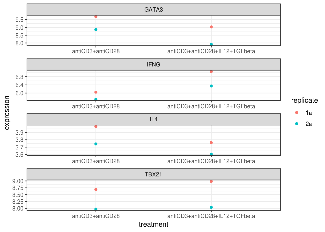

Figure 4.1: Expression level vs. treatment

4.9 Differential expression analysis

Now we’ll take our new genes-only expression data and put it into a form expected by limma.

eset_genes <- eset_tib_genes_only %>%
  as.data.frame() %>%
  column_to_rownames(var="first_gene_symbol") %>%
  data.matrix() %>%
  ExpressionSet()

One last step: we need to make the design matrix for this comparison.

treatments <- factor(c(1,2,2,1), labels=c("untreated", "treated")) # weird ordering of files
design <- model.matrix(~treatments)

Finally we use limma to perform a differential expression analysis!

fit_genes <- lmFit(eset_genes, design)
fit2_genes <- eBayes(fit_genes)
results_genes <- topTable(fit2_genes, number=Inf)
results_genes_tib <- as_tibble(results_genes, rownames = "gene")

Let’s look at our results.

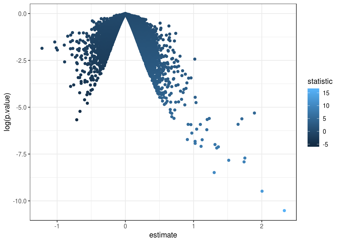
Figure 4.2: Volcano plot made with biobroom

References

Godec, Jernej, Yan Tan, Arthur Liberzon, Pablo Tamayo, Sanchita Bhattacharya, Atul J Butte, Jill P Mesirov, and W Nicholas Haining. 2016. “Compendium of Immune Signatures Identifies Conserved and Species-Specific Biology in Response to Inflammation.” Immunity 44 (1): 194–206.